From WLAN to W-CDMA, all wireless devices have one thing in common, that is, there is no wired connection. Signals transmitted through the air are distorted by atmospheric damage, disrupted by natural and man-made obstacles, and further by the relative movement of the transmitter and receiver. This process is called fading. Fading is inevitable in real-world environments, so wireless communication systems must be able to handle this problem while maintaining accurate data transmission capabilities.
Simulating the fading damage of the actual channel is critical to the testing of wireless devices. To accurately perform channel simulation, different fading scenarios and their effects must be understood and mathematical models of these fading effects must be created. Agilent Technologies offers a new solution for simulating fading during wireless device testing, mitigating some of the most difficult and costly challenges in channel emulation.
Before considering a solution, it is important to understand the different manifestations of fading. The different manifestations of fading have different causes, and they affect the channel in various ways.
Cause of declineThe ability to successfully communicate between the transmitter and the receiver depends to some extent on the fading characteristics of the channel in which the signal propagates. Wide range fading includes the effect of signals traveling over long distances (several hundred or more wavelengths). The small range fading mechanism affects the signal near the receiver.
Wide-range fading includes the average attenuation of the signal over a distance (in the ideal line-of-sight propagation (LOS) condition, which is proportional to the square of the distance), and the diffraction of the signal caused by large objects such as mountains or skyscrapers.
Small-range fading is the result of both multipath propagation and Doppler shift. Multipath fading occurs because the transmitted signal causes reflection, diffraction, and local scatter when it encounters mailboxes, trees, and moving vehicles, and arrives at the receiver through different paths. Therefore, the receiver obtains multiple copies of the signal at different arrival times (see Figure 1). These copies are received at different phase and power levels, causing signals to interfere with each other and cause power fluctuations.

Figure 1. Multipath fading occurs when a transmitted signal encounters various objects on the path to the receiver, causing it to reach the receiver at slightly different times.
Doppler shift fading is the result of movement. If the receiver is moving relative to the transmitter, the frequency of the signal entering the receiver will vary depending on the direction and speed at which the receiver moves relative to the transmitter. A copy of the signal arriving along the path directly in front of the receiver will detect a higher frequency than the transmitted signal, and a copy of the signal arriving along the path behind the mobile receiver will have a lower detected frequency.
Therefore, multipath reflection and Doppler shift change (fade) the transmitted signal, making it difficult for the receiver to accurately understand the signal. These effects vary depending on the channel environment (urban or rural), signal wavelength, and relative movement of objects in the transmitter/receiver and environment.
Fading classificationOne of the effects of multipath propagation is the time spreading of the signal such that the first signal on the shortest path from the receiver is copied to the last signal copy it receives on the longest path with a limited delay. The maximum delay is expressed in Tm (Figure 2a).
In the frequency domain, time broadening can be described as a frequency dependent function. This function represents the degree of correlation between the impulse responses of the two signals. The coherence bandwidth (f0) is the frequency range in which the signal impairment of the channel does not change significantly (Fig. 2b). F0 is inversely proportional to Tm.

Figure 2. Effect of time distribution on the channel: a) maximum delay; b) coherence bandwidth.
Multipath fading can affect mobile receivers or fixed receivers. Mobile receivers and receivers operating in channels containing moving objects must also handle other factors that affect signal amplitude and phase. These effects can be described as a function of time or spatial variation. If the receiver moves at a constant speed, sending pulses at different times is exactly the same as sending pulses at different locations.
When transmitting signals on a varying channel, it is important to know how long these conditions are stable. This is called the coherence time (T0) (Figure 3a). T0 can also be considered as the length of time that is highly correlated with the impulse response of the channel.
We can also view time changes in the frequency domain. The receiving opportunity that is moving all the time is subject to frequency shift, which depends on the angle of arrival of the received signal. Time broadening causes the signal to broaden over time; changes in time (or space) cause the signal to broaden in frequency. The receiver does not get a signal at one frequency, but instead gets different parts of the signal at different frequencies. This Doppler broadening (fd) is inversely related to the coherence time T0 (Fig. 3b).
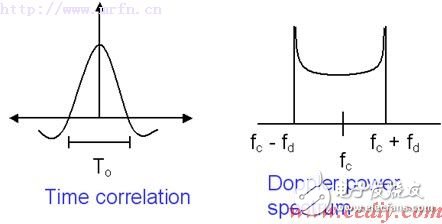
Figure 3. Effect of time variation on the channel: a) coherence time; b) Doppler broadening.
In summary, small-scale fading appears as time broadening (delay broadening) or time variation (Doppler broadening). (If the receiver is moving, the signal may experience both fading at the same time.) These two fading can be further classified according to the fading variation with frequency or time. The characteristics of these fading are listed below.
Time broadening: flat decline
· The time to transmit a symbol is greater than the maximum delay spread (Ts "Tm).
· The signal bandwidth is less than the coherence bandwidth (B “f0â€).
· Receive all multipath components in one symbol period.
Time broadening: frequency selective fading
· The time to transmit a symbol is less than the maximum delay spread (Ts "Tm").
· The signal bandwidth is greater than the coherence bandwidth (f0 ′ B).
• The channel changes the different spectral components of the signal in different ways, so the received power of the wideband signal may vary greatly with frequency over its bandwidth.
Time change: fast fading
· The symbol period is longer than the coherence time (Ts T0).
· The signal bandwidth is less than the Doppler spread (B “fdâ€).
· The channel fading condition changes faster than the symbol is sent.
Time change: slow fading
· The symbol period is shorter than the coherence time (Ts "T0").
· The signal bandwidth is greater than the Doppler spread (B ′ fd).
· Channel conditions are stable and predictable during symbol transmission.
Impact of fadingLarge-scale fading mainly leads to level fading of the overall signal. Path attenuation is extremely dependent on distance. Its effect on the device is to reduce the signal-to-noise ratio (SNR) by reducing the received signal power. The shadow effect and the wide range of reflections appear as deviations in this average path attenuation.
Small-scale fading caused by multipath and Doppler effects may be the most destructive to communication. Frequency selective fading can lead to inter-symbol interference (ISI), making it more difficult to accurately understand the received symbols. Flat fading can degrade the SNR because reflection causes the vector components to cancel each other out. Fast fading can distort the transmitted baseband data pulses, which can cause phase-locked loop synchronization problems. Slow fading also reduces SNR. The reduction in SNR requires the designer of the wireless device to increase the "fading margin" when determining the link requirements; the signal power must be strong enough, or the sensitivity of the receiver should be high enough to function properly in a fading situation.
Reduce the effects of fadingThe ideal wireless link performance can only be achieved without channel impairments. However, the presence of additive white Gaussian noise (AWGN) makes it impossible for the wireless channel to be completely undisturbed. However, many techniques can be employed to design wireless devices to reduce the effects of fading. These techniques reduce the bit error probability of the worst-case fading curve, making it closer to the best-case AWGN curve. Different forms of fading have different effects on the bit error rate. Frequency selective fading and fast fading can significantly affect the bit error rate, while flat fading and slow fading have less effect on the bit error rate. Determining the type of fading in a channel is very important when designing a wireless link that can tolerate fading to signal degradation. Then, you can choose the information rate and reduce the number of errors that can be avoided.
Since the symbol frequency is inversely related to the symbol period, changing the signal rate to compensate for frequency selective fading also changes its performance in terms of fading speed. To avoid frequency selective fading, the transmission rate should be lower than the coherence bandwidth of the channel (B "f0"). However, in order to reduce the distortion caused by fast fading, it is important to set the transmission rate to be greater than the channel fading rate (B ′ fd). In other words, frequency selective fading determines the upper limit of the signal bandwidth, and fast fading determines the lower limit of the signal bandwidth.
Equalization is a common technique used to eliminate ISI caused by frequency selective fading. This process is to call a filter with an impulse response opposite to the propagation channel. Therefore, the transmission channel is combined with the receive filter to produce a flat linear response. For example, GSM uses adaptive equalization techniques to mitigate distortion.
CDMA technology uses the Raker receiver to mitigate the effects of ISI. The Raker receiver uses a dedicated filter to detect the components in the stretched signal, collect the components, and cohere them together (using a delay longer than the late path for the early arrival path).
We can also use interleaving techniques and coding techniques to reduce the Eb/No (energy-to-noise ratio) required to accurately detect signals. Encoding techniques provide redundancy by transmitting multiple copies of the signal on orthogonal code channels. The interleaving technique adds stability to the link by distributing the errors to different times, thereby avoiding a large number of consecutive data loss phenomena, which may cut off the wireless link.
Some transmission technologies have signal characteristics that avoid the most common effects of fading. For example, ultra-wideband transmission technology, which transmits a pulse period that is so short that it is not affected by channel delay broadening. Orthogonal Frequency Division Multiplexing (OFDM) avoids frequency selective fading by dividing the carrier signal into subcarriers with lower information rates.
Fading curveFading in some way hinders signals propagating through the wireless channel. In order to design a device that can tolerate such damage, it is important to use tools that can simulate fading in a laboratory environment. These tools create fading effects in real-world environments by mathematically generating conditions that simulate large-scale fading and small-scale fading. These mathematical expressions are based on certain mathematical models that use statistical data to predict how electromagnetic waves behave during propagation. Some typical fading models are described below.
Large-scale fading can be mathematically simulated by superimposing the signal fluctuations of the lognormal distribution over the average path attenuation associated with the distance. For large-scale fading, the most accurate channel simulation equations are derived from empirical formulas derived from measurements taken in specific urban areas and obtained.
The Rayleigh distribution is a good channel propagation model when there is no strong line-of-sight propagation path between the transmitter and receiver. It can properly represent the channel conditions in the urban area, where the building blocks the line-of-sight propagation path, and the signal is broadened at the receiving end after being reflected by various objects. In the time domain, Rayleigh fading has a period peak (depth fading) of no more than 10 dB between slots of 40 dB or more (Figure 4a).
In the frequency domain, the Rayleigh distribution produces a U-shaped curve (Figure 4b). The dense scattering model can be used to describe the case of cellular communications, which means that the amplitude of the multipath signal will exhibit a Rayleigh distribution and the angle of arrival (multipath phase) will exhibit a normal distribution.
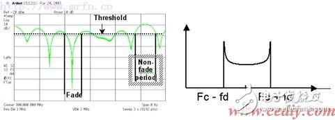
Figure 4. Rayleigh distribution: a) time domain; b) frequency domain.
In the rural environment, there are fewer objects blocking the signal. The multipath signal includes a strong line-of-sight propagation path and a small number of reflection paths, and the spectrum power is a Rician distribution. The angle of arrival of the direct path and the ratio of the power between the direct path and the other path determine how much energy from the direct path affects the normal Rayleigh model of multipath fading. The graph in the frequency domain looks like a Rayleigh distribution, but at the frequency shift caused by the direct path, the power has a peak. (Figure 5)
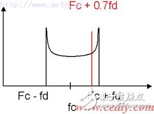
Figure 5. Rice distribution (frequency domain).
The Suzuki fading curve combines small-scale fading caused by multipath propagation with large-scale fading caused by reflection and diffraction. Large-scale fading is log-normally distributed, and small-range fading is Rayleigh distribution (Fig. 6).

Figure 6. Suzuki curve.
Fading curve depends on the signal environmentThe impulse response of the propagation channel is heavily dependent on the user environment. When a signal travels through the air, it encounters objects of all sizes and therefore reaches the receiver through various paths. Each path has a different distance, so the received signal fluctuates in amplitude and phase. When the transmitted energy encounters an obstruction, the latter case depends on the size and density of the obstruction compared to the wavelength of the incident signal. When an electromagnetic wave encounters a large, smooth object that is much larger than the wavelength (such as a concrete-built building), the signal is reflected or diffracted. If an electromagnetic wave encounters an object whose size is a wavelength level (such as a street sign, leaves, or a smog), it will scatter evenly in all directions. An omnidirectional antenna is capable of receiving a small number of bits that appear to be scattered signals from various directions. The magnitude of these scattered signals follows the probability density function described by the Rayleigh distribution.
When there is a strong direct path, the amplitude will be closer to the Rice distribution curve. This is the most accurate in the rural environment. In rural environments, there are relatively few obstacles, thus allowing a strong direct path to be established from the base station to the mobile station. The Rice model is also a good choice for satellite communications testing because these systems include strong direct paths and atmospheric attenuation and scattering.
If the receiver is moving, it will widen the frequency of the multipath signal arriving at the receiver. As the speed increases, the frequency shift also increases. The frequency shifting of the multipath signal results in a frequency broadening, or fading rate fd.
If the antenna moves in an indoor environment, it will also experience Doppler broadening. However, the resulting power spectrum is not a normal U-shaped curve, but a flat curve that looks like a long right angle. The shape of this change is primarily the result of multi-channel reflections from the ceiling, and it is clear that this does not happen in outdoor environments.
Fading testTesting whether a wireless system (including mobile stations and base stations) can successfully transmit and receive data in a fading situation is an important part of the detection process. Wireless standards generally specify extensive and detailed fading tests. Currently, the channel emulation method used to implement fading testing is a challenging process.

Figure 7. The current channel emulation method reduces accuracy during analog-to-digital conversion.
The current channel emulation method starts from the RF signal and ends with the RF signal (Figure 7). Test signals that require simulated fading are downconverted and digitized. The fading curve is then combined in the digital signal and the result is then upconverted back to RF. Finally add noise. (Note: AWGN is independent of multipath effects and must be added separately.)
This method involves two processes: conversion loss and noise calibration. These two processes result in inefficiencies and poor accuracy. When the simulated signal is converted to a digital signal or a digital signal is converted into an analog signal, the test device (rather than the channel or device under test) introduces an error. This conversion loss increases measurement uncertainty.
Determining the amount of noise to increase to achieve a certain carrier-to-noise ratio (C/N) is a difficult process. We require that AWGN be added to the signal after the simulation fades, so that it will not be attenuated and deviate from the desired signal level. However, increasing this noise causes the total power level to deviate from the total power level after fading, while changing the C/N ratio. It is therefore necessary to calculate the carrier power after fading to determine the corresponding noise level to be increased when the input signal power is constant, which is a complicated, time consuming, and costly process.
Channel simulation integration technologyAgilent has developed a new channel emulation technology for R&D engineers who are designing digital devices for wireless devices. It reduces design detection time with faster, more accurate channel simulation. This new approach enhances the capabilities of the industry-leading E4438C ESG vector signal generator, providing an intuitive software interface while providing best-in-class baseband generation hardware. ESG creates digital baseband IQ signals using built-in cellular communication models, Signal Studio applications, or custom waveforms created by mathematical modeling tools such as Agilent Eesof's Advanced Design System (ADS) or MATLAB®. These digital baseband signals are sent to a PC containing the Baseband Studio PCI card and Baseband Studio fading software. Users can configure channel emulation parameters on the PC through an easy-to-use software interface. The baseband signal is digitally faded in the Baseband Studio PCI card and then sent back to the ESG for conversion to a simulated I/Q or RF signal output.
Simulating different fading curves is a basic requirement for evaluating receiver performance in a variety of environments. Baseband Studio fading software can simulate large range fading, small range fading, or a combination of both. It simulates rapid signal fluctuations due to small displacements of the receiver and slow changes in average power due to shadowing effects of remote objects. The fading curves it supports include:
· Lognormal distribution - wide range direct path loss
· Rayleigh distribution - small-range multipath scattering
· Rice distribution - Rayleigh distribution with direct path
· Suzuki distribution - Rayleigh distribution with lognormal distribution
· Pure Doppler effect - Doppler shift due to movement
User-defined fading curves can be flexibly adapted to specific test needs. You can adjust the relationship between the number of multipaths and the available bandwidth to maximize processing power and achieve test flexibility. It is implemented on an extremely accurate instrument platform, and the entire fading process is implemented on a digital baseband, improving test accuracy. You can also add two channels to simulate a diversity antenna or an interfering signal. You can simplify the initial setup with standard fading curves such as pre-configured W-CDMA, TD-SCDMA, cdma2000, cdmaOne, 1xEV-DO, 1xEV-DV, GSM, EDGE, and WLAN.
In addition, Agilent offers pre-defined settings for commonly used cellular systems, which also simplifies test preparation. These curves can be modified to provide a tailored configuration for simulating specific environments. The pre-defined settings also include 3GPP W-CDMA's unique mobile propagation conditions and birth and fall fading curves.

Figure 8. The new Agilent fading scheme supports user-defined flexibility.
Figure 8 is a general block diagram of Agilent's new fading solution. A pair of I/Q input signals are routed to up to N different signal processing paths, simulating up to N different RF propagation paths. The delay module adds user-defined delays on each path in very fine increments (a fraction of a nanosecond). The complex multiplication module combines the delay information with the fading information provided by the fading algorithm in the DSP. The fading algorithm uses a user-specified fading curve for the input I and Q data. Finally, these paths are superimposed to generate an I/Q baseband data stream that is then input to the ESG and upconverted by the ESG to RF.

Figure 9. Block diagram of the DSP fading algorithm.
Figure 9 illustrates a DSP algorithm that uses fading to form fading. The complex random noise with a Gaussian distribution has the magnitude of the Rayleigh distribution. The amplitude table converts the normal distribution noise in the random number generator into a Rayleigh distribution. The phase table converts the normally distributed noise input representing the phase into appropriate I and Q values, generating a unit vector for that phase.
Rice's fading is only Rayleigh's fading plus an additional unfading direct path that produces a Doppler shift relative to the Rayleigh fading signal. For the Rice fading curve, in addition to the Doppler broadening, the Doppler module adds a rotating constant amplitude vector (Doppler shift) to the fading signal before it enters the complex multiplication module.
Full digital fading simulation to reduce errorsAs mentioned earlier, the traditional process of fading simulation is to digitize the input RF signal, then fading the signal, and then upconverting back to RF. This adds a very large amount of uncertainty to the entire process. This uncertainty is due to nonlinear distortion, balance error, clipping, sampling misunderstanding, carrier feedthrough, and other problems in the DAC. All of these potential errors must be considered when testing new wireless devices.
One way to reduce digitization errors is to increase the resolution of the digitizer and use a higher data rate to better approximate the original analog signal. But the best solution is to avoid unnecessary analog to digital conversions. If the signal generator's raw digital I/Q output is used to digitally complete the entire process, these errors can be significantly reduced. Signal fading is performed with an all-digital process that reduces the added errors of the normal analog-to-digital conversion process.
Built-in AWGN generator reduces costsTraditional fading simulators do not have built-in AWGN functionality, requiring additional calibration of signal levels. Adding AWGN to a fading signal typically causes problems when setting the desired signal-to-noise ratio because we have to combine two different RF signals to achieve the desired overall signal level and ratio.
By using the Baseband Studio fading software, you can change the noise value by inputting the C/N or Eb/No value on the user interface. At the same time, C, N, C/N or C+N can be kept unchanged, simplifying the receiver performance. Test. Baseband Studio fading software obtains power level and data rate information from the ESG and automatically changes the signal without requiring separate adjustments to the carrier and noise power.
Baseband Studio fading software seamlessly integrates with the E4438C ESG, eliminating calibration issues associated with traditional fading simulators. The baseband signal from the ESG (16-bit digital signal) is sent to the Baseband Studio fading software, which adds multipath fading and AWGN to the original baseband data, all in the digital domain. In fact, the entire channel emulation process remains in digital form until the signal is upconverted to RF. It achieves excellent carrier-to-noise ratio accuracy because it eliminates the uncertainty associated with increasing the simulated signal.
Accurate and economical simulation of fading is critical to the effective testing of wireless devices. Agilent's Baseband Studio fading software in an integrated environment simplifies wireless testing and helps you get to market faster.
24V Battery Pack ,Large Battery Pack,24 V Battery Pack,24V Lithium Ion Battery Pack
Zhejiang Casnovo Materials Co., Ltd. , https://www.casnovo-new-energy.com